Plot Method for bbnp_regression Objects — plot.bbnp

Creates visualizations of bias-bounded conditional expectation estimation results

Usage

# S3 method for class 'bbnp_regression'
plot(
  x,
  type = c("regression", "ft"),
  fill_ci = .bbnp_pal[["ci"]],
  alpha_ci = 0.55,
  point_alpha = 0.28,
  point_color = .bbnp_pal[["point"]],
  ft_resol = 500,
  xi_range = NULL,
  expand = 2.5,
  ...
)

Arguments

x

An object of class bbnp_regression

type

Character string specifying plot type. Options are:

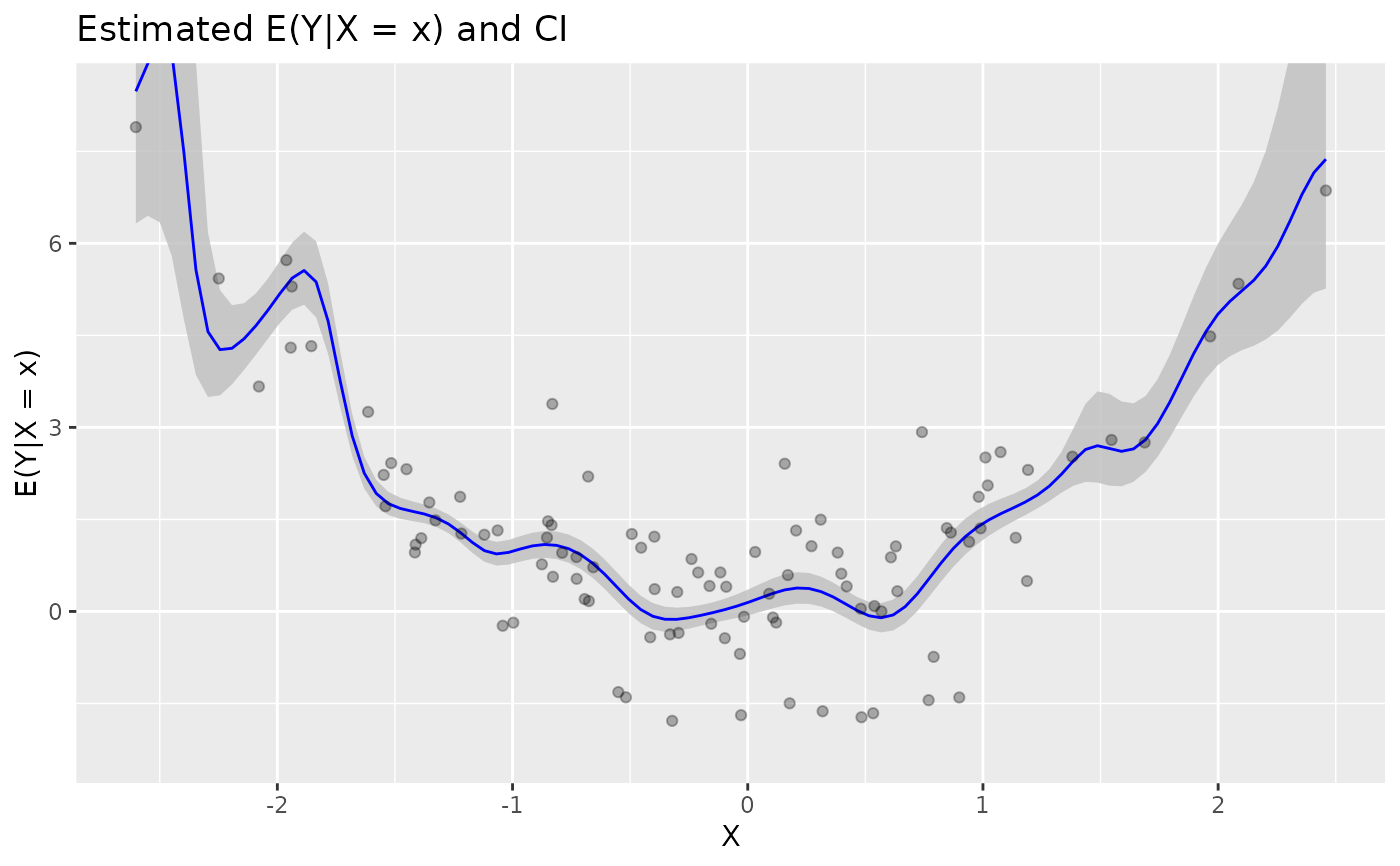
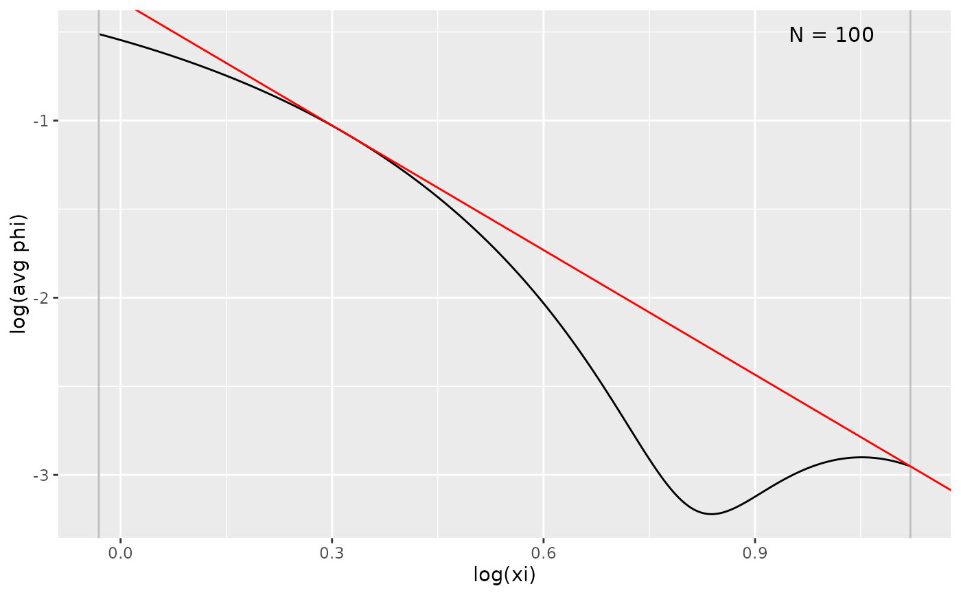
"regression" (default): Conditional expectation with confidence interval
"ft": Fourier transform plot with estimated envelope

fill_ci

Color for confidence interval ribbon (default: a muted blue).

alpha_ci

Transparency for confidence interval ribbon (default: 0.35)

point_alpha

Transparency for data points (default: 0.28)

point_color

Color for data points (default: a soft grey).

ft_resol

Resolution for Fourier transform plot (default: 500)

xi_range

Optional numeric c(lower, upper) giving the frequency range to display in the "ft" plot. If NULL (default) a wide range around the selected window is shown (see expand). This controls only what is drawn; it does not change the fitting window [xi_lb, xi_ub].

expand

For the "ft" plot when xi_range is NULL: how far past the selected window to display, as a multiple (default 2.5).

...

Additional arguments (unused)

Value

A ggplot2 object

Examples

# \donttest{
X <- gen_sample_data(size = 500, dgp = "2_fold_uniform", seed = 1)
Y <- 2 * X - X^2 + rnorm(length(X), sd = 0.3)
fit <- biasBound_condExpectation(Y, X, h = 0.1)
plot(fit)

plot(fit, type = "ft")

# }