Density Estimation with rbbnp

This article is a guide to density estimation with biasBound_density().

Estimating a density

biasBound_density() takes a data vector and returns a density estimate with bias-aware confidence intervals. The main arguments are:

biasBound_density(
  X,                    # Data vector
  x = NULL,             # Evaluation points (auto if NULL)
  h = NULL,             # Bandwidth (auto-selected if NULL)
  h_method = "cv",      # "cv" or "silverman"
  alpha = 0.05,         # Confidence level
  kernel.fun = "Schennach2004",
  xi_lb = NULL,         # Frequency range lower bound
  xi_ub = NULL          # Frequency range upper bound
)

A basic fit, on data drawn from the 2-fold uniform distribution:

# Generate sample data from 2-fold uniform distribution
X <- gen_sample_data(size = 1000, dgp = "2_fold_uniform", seed = 42)

# Estimate density
fit <- biasBound_density(X, h = 0.08, kernel.fun = "Schennach2004")

# Display results
fit
#> Bias-Bounded Density Estimation
#> 
#> Call:
#> biasBound_density(X = X, h = 0.08, kernel.fun = "Schennach2004")
#> 
#> Sample size: n = 1000
#> Bandwidth:   h = 0.0800 (user-specified) 
#> Kernel:      Schennach2004 
#> 
#> Bias bound parameters:
#>   A = 6.8980, r = 2.5142
#>   bias bound b1x = 0.0334
#> 
#> Evaluation points: 100 (range: [-0.1746, 2.1780])
#> Confidence level: 95%
#> 
#> Use summary() for detailed statistics
#> Use plot() to visualize results

The result is an S3 object of class bbnp_density. Use coef() for the key parameters and summary() for a fuller report:

# Key parameters
coef(fit)
#>        A        r        h 
#> 6.898006 2.514158 0.080000

# Detailed summary
summary(fit)
#> Summary: Bias-Bounded Density Estimation
#> ============================================================
#> 
#> Call:
#> biasBound_density(X = X, h = 0.08, kernel.fun = "Schennach2004")
#> 
#> Sample Information:
#>   Sample size (n):  1000
#>   Bandwidth (h):    0.0800
#>   Kernel function:  Schennach2004
#> 
#> Bias Bound Parameters:
#>   A (amplitude):    6.8980
#>   r (decay rate):   2.5142
#>   b1x (bias bound): 0.0334
#>   Xi interval:      [2.4074, 4.5544]
#> 
#> Range Estimation:
#>   Density estimates:
#>    min Q1.25% median   mean Q3.75%    max 
#> 0.0000 0.1111 0.4273 0.4217 0.7125 0.8798 
#> 
#>   Standard errors:
#>    min   mean    max 
#> 0.0000 0.0341 0.0563

Visualizing the fit

The default plot shows the estimate together with the bias band and the confidence interval:

plot(fit)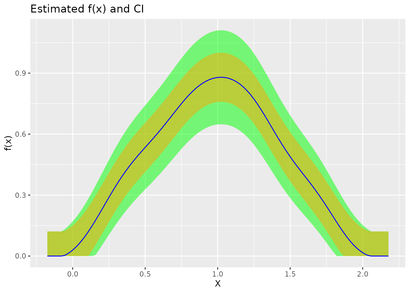

Element	Description
Estimate	Kernel density estimate \(\hat{f}(x)\)
Bias bound	Bias range: \([\hat{f} - \bar{b}, \hat{f} + \bar{b}]\)
95% CI	\([\hat{f} - \bar{b} - z\hat{\sigma}, \hat{f} + \bar{b} + z\hat{\sigma}]\)

The type = "ft" plot shows how the smoothness parameters are detected from the empirical Fourier transform:

plot(fit, type = "ft")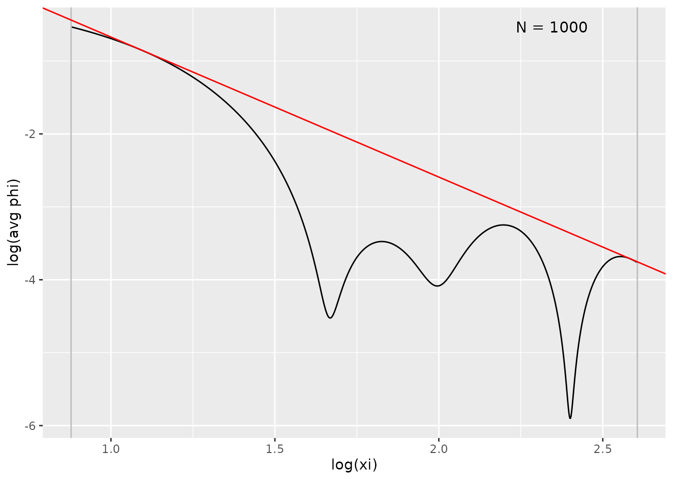

The legend labels each line:

Empirical |phi|: the empirical Fourier transform \(|\hat{\phi}(\xi)|\)
Fitted envelope: the estimated envelope \(A|\xi|^{-r}\), drawn over the selected window
Shaded band: the selected frequency range \([\underline{\xi}, \bar{\xi}_n]\)

The slope \(r\) measures smoothness: a larger \(r\) means a smoother function.

Choosing the bandwidth

When h is left NULL, the bandwidth is selected automatically by the method named in h_method. Cross-validation is the default:

fit_cv <- biasBound_density(X, h = NULL, h_method = "cv", kernel.fun = "normal")
cat("CV bandwidth:", coef(fit_cv)["h"], "\n")
#> CV bandwidth: 0.1878156

plot(fit_cv) + ggtitle("Cross-Validation Bandwidth")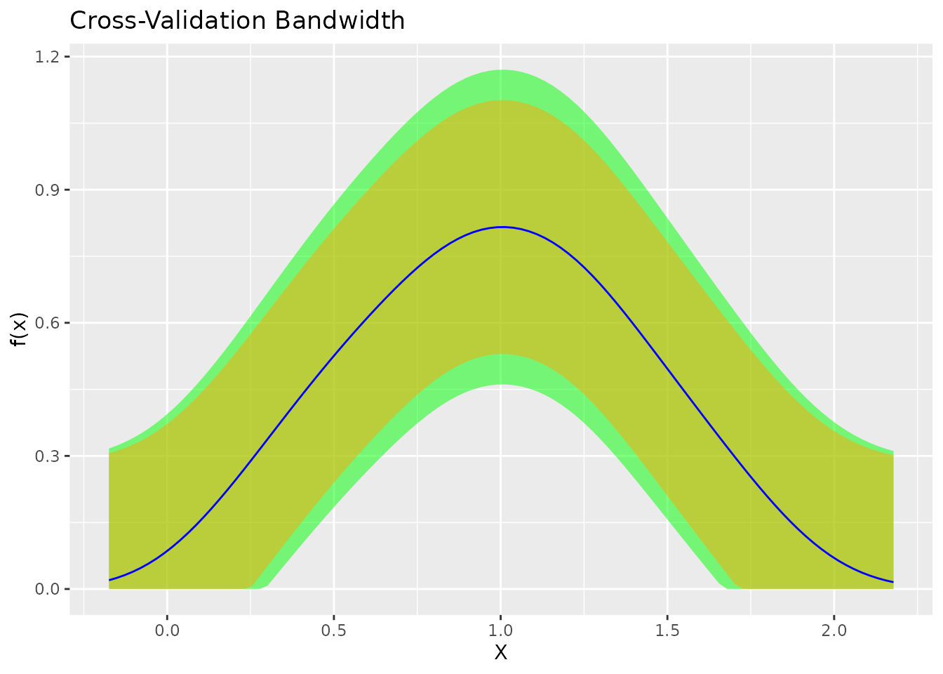

Silverman’s rule of thumb is a faster alternative:

fit_silv <- biasBound_density(X, h = NULL, h_method = "silverman", kernel.fun = "normal")
cat("Silverman bandwidth:", coef(fit_silv)["h"], "\n")
#> Silverman bandwidth: 0.09390781

plot(fit_silv) + ggtitle("Silverman's Rule Bandwidth")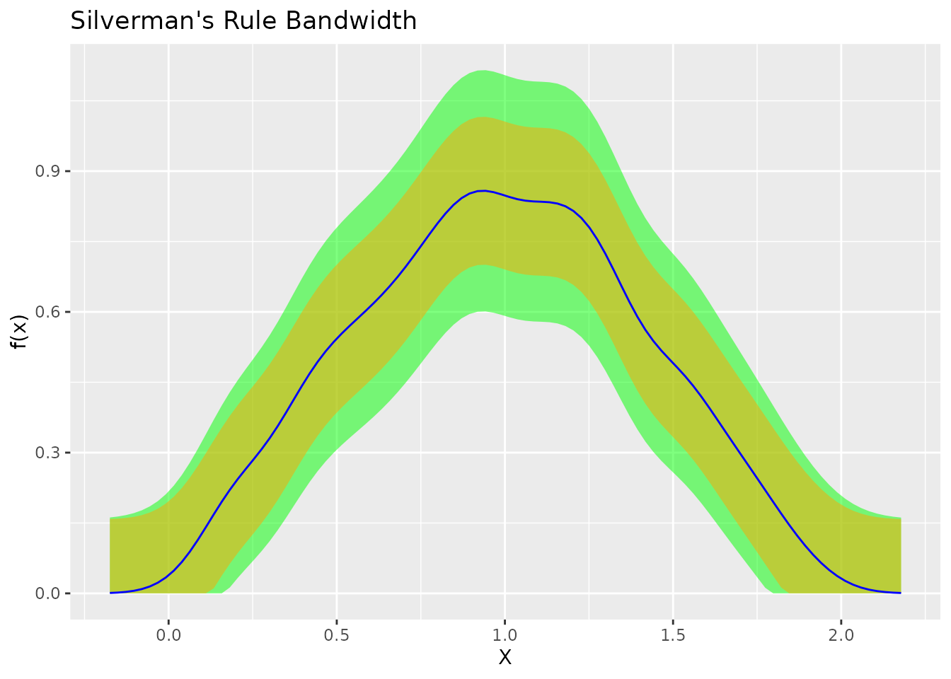

To obtain a bandwidth on its own, without fitting, call select_bandwidth():

# Select bandwidth without full estimation
h_cv <- select_bandwidth(X, method = "cv", kernel.fun = "normal")
h_silv <- select_bandwidth(X, method = "silverman", kernel.fun = "normal")

cat("CV:", h_cv, "\nSilverman:", h_silv)
#> CV: 0.1878156 
#> Silverman: 0.09390781

Kernel functions

Four kernels are available, differing in their order and the smoothness they suit:

Kernel	Order	Best For
Schennach2004	Infinite	High smoothness (recommended)
sinc	Infinite	Any smoothness level
normal	2	Moderate smoothness
epanechnikov	2	Limited smoothness

The same data fitted with each kernel:

fit_sch <- biasBound_density(X, kernel.fun = "Schennach2004")
fit_sinc <- biasBound_density(X, kernel.fun = "sinc")
fit_norm <- biasBound_density(X, kernel.fun = "normal")
fit_epan <- biasBound_density(X, kernel.fun = "epanechnikov")

grid.arrange(
  plot(fit_sch) + ggtitle("Schennach2004 (infinite order)"),
  plot(fit_sinc) + ggtitle("Sinc (infinite order)"),
  plot(fit_norm) + ggtitle("Normal (2nd order)"),
  plot(fit_epan) + ggtitle("Epanechnikov (2nd order)"),
  ncol = 2
)

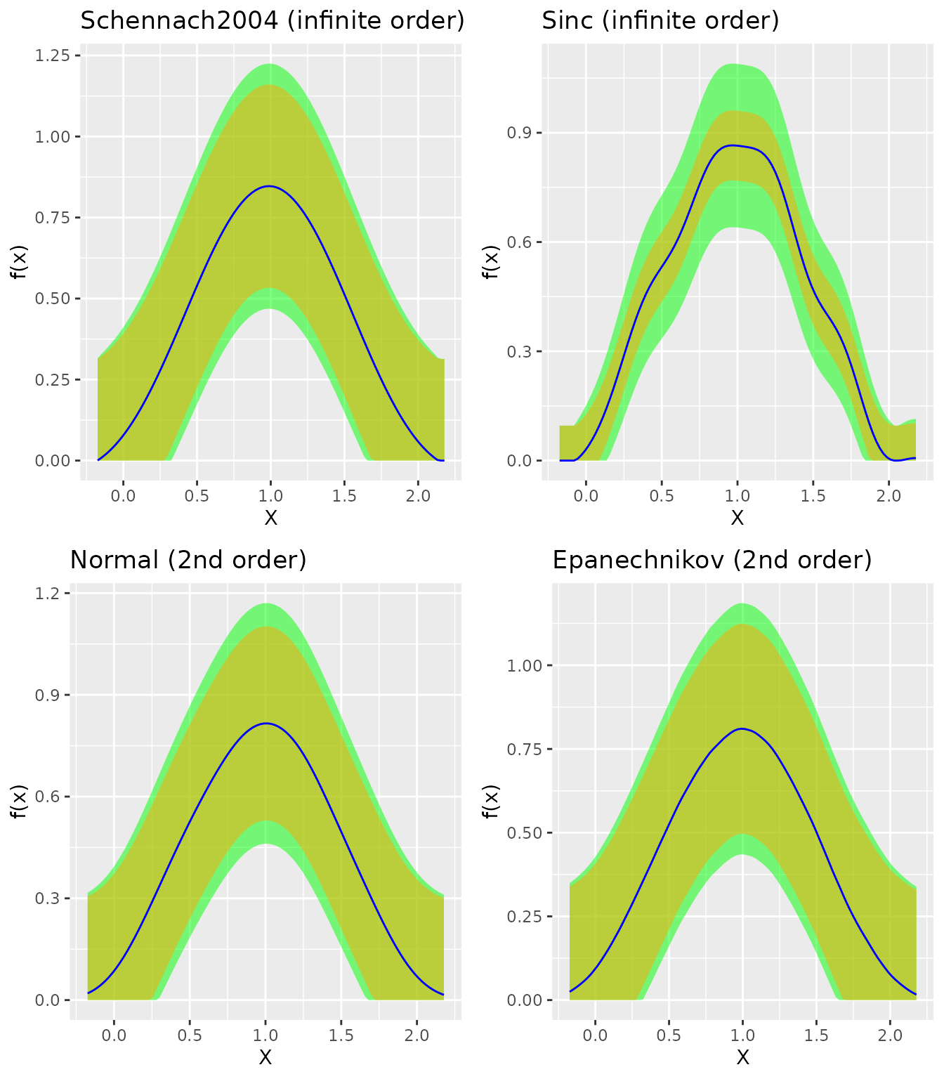
For most applications use "Schennach2004", which adapts to any smoothness level.

Bias and the bandwidth tradeoff

Changing the bandwidth moves the two pieces of the interval in opposite directions. A larger bandwidth lowers the variance (the sampling band narrows) but raises the bias (the bias band widens); a smaller bandwidth does the reverse. The plots below show the same data at the optimal bandwidth and at half of it:

h_opt <- select_bandwidth(X, method = "cv", kernel.fun = "sinc")

# Bias-bound interval at the optimal bandwidth
result_opt <- biasBound_density(X, h = h_opt, kernel.fun = "sinc")

# ... and at a smaller (undersmoothed) bandwidth
result_under <- biasBound_density(X, h = h_opt * 0.5, kernel.fun = "sinc")

grid.arrange(
  plot(result_opt) + ggtitle(paste0("Optimal bandwidth (h = ", round(h_opt, 3), ")")),
  plot(result_under) + ggtitle(paste0("Undersmoothed (h = ", round(h_opt/2, 3), ")")),
  ncol = 1
)

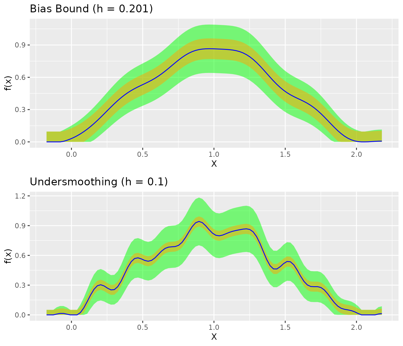
At the optimal bandwidth the bias band is the larger component, so the total interval here is wider than at the undersmoothed bandwidth. That is expected. The optimal bandwidth delivers valid inference at the MSE-minimizing variance rate, and a single sample can still produce a wide band. The Theoretical Background article explains why a naive interval at the optimal bandwidth under-covers, and why undersmoothing, the classical alternative, is asymptotically inefficient.

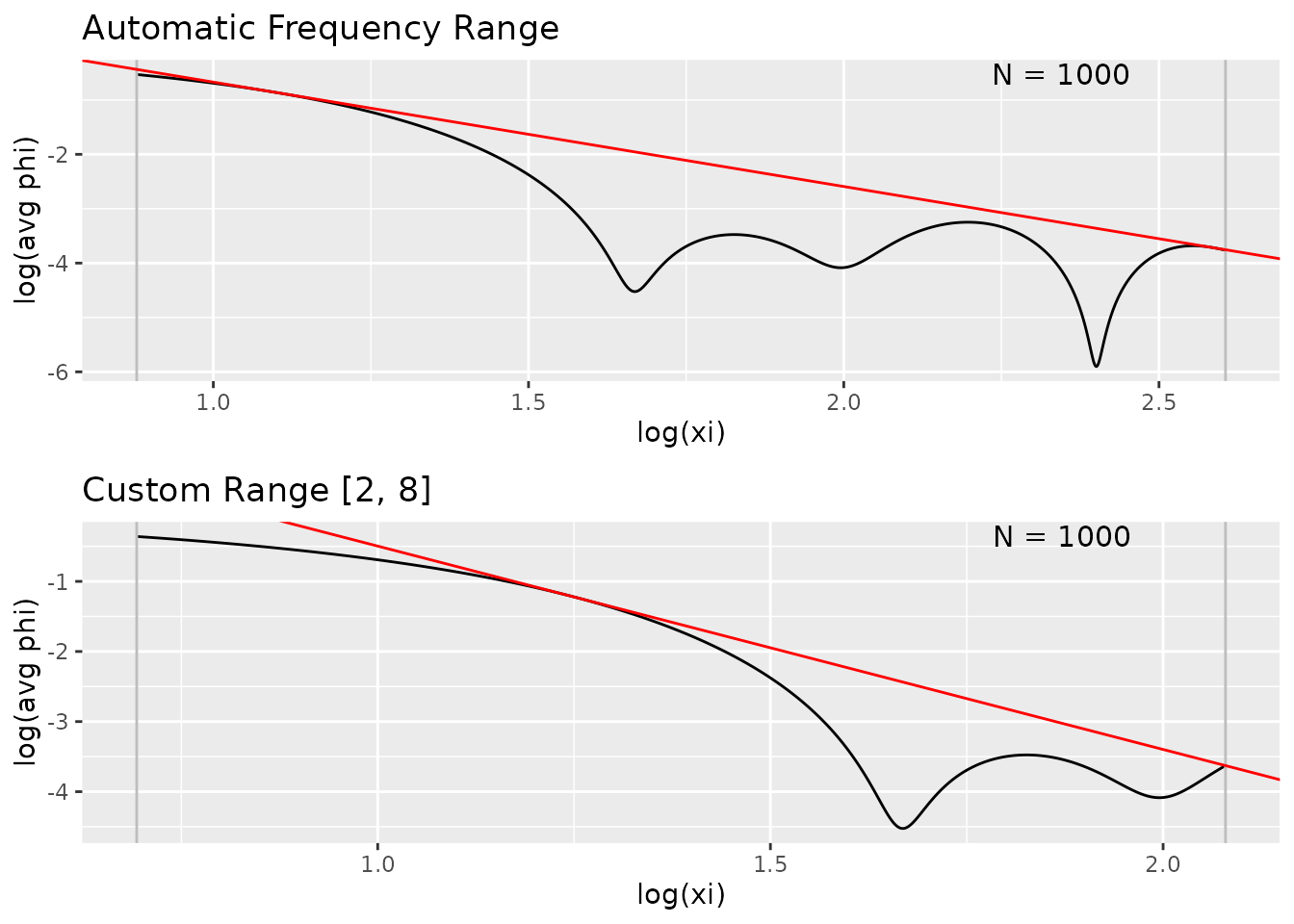
More options

You can set the Fourier frequency window by hand with xi_lb and xi_ub, instead of letting the package choose it:

# Default (automatic)
fit_auto <- biasBound_density(X, h = 0.08)

# Custom range
fit_custom <- biasBound_density(X, h = 0.08, xi_lb = 2, xi_ub = 8)

grid.arrange(
  plot(fit_auto, type = "ft") + ggtitle("Automatic Frequency Range"),
  plot(fit_custom, type = "ft") + ggtitle("Custom Range [2, 8]"),
  ncol = 1
)

The estimate, evaluation grid, and confidence intervals are all available on the fitted object:

# Confidence intervals as matrix
ci <- confint(fit)
head(ci, 10)
#>       lower      upper
#>  [1,]     0 0.03341978
#>  [2,]     0 0.03341978
#>  [3,]     0 0.03341978
#>  [4,]     0 0.03341978
#>  [5,]     0 0.03341978
#>  [6,]     0 0.04274476
#>  [7,]     0 0.05896604
#>  [8,]     0 0.07625691
#>  [9,]     0 0.09584398
#> [10,]     0 0.11785186

# Evaluation points
x_points <- fit$x
head(x_points)
#> [1] -0.1746134 -0.1508492 -0.1270850 -0.1033208 -0.0795566 -0.0557924

# Density estimates
f_hat <- fit$density
head(f_hat)
#> [1] 0.000000000 0.000000000 0.000000000 0.000000000 0.000000000 0.002945549