Theoretical Background

This article gives the mathematical background for the bias-bound approach, based on Schennach (2020).

The bias-variance tradeoff

In nonparametric estimation we face a fundamental tradeoff:

Large bandwidth: low variance but high bias
Small bandwidth: low bias but high variance

Traditional approaches take one of two routes:

Undersmooth: use a smaller bandwidth to reduce bias, which inflates variance and produces inefficient confidence intervals
Ignore bias: use the optimal MSE bandwidth but produce invalid confidence intervals

The bias-bound approach takes a third route: it bounds the bias. This lets you use the optimal MSE-minimizing bandwidth, construct confidence intervals that account for the potential bias, and keep valid coverage without sacrificing efficiency.

A Fourier view of the bias

For a sample \(X_1, \ldots, X_n\) from a density \(f\), the kernel density estimator is

\[\hat{f}_h(x) = \frac{1}{nh} \sum_{i=1}^{n} K\left(\frac{x - X_i}{h}\right)\]

where \(K\) is the kernel and \(h\) is the bandwidth. Its error splits into two parts:

\[\hat{f}_h(x) - f(x) = \underbrace{[\hat{f}_h(x) - E[\hat{f}_h(x)]]}_{\text{variance term}} + \underbrace{[E[\hat{f}_h(x)] - f(x)]}_{\text{bias term}}\]

The variance term is random with a known distribution. The bias term is deterministic but unknown, and the method must control it.

The bias-bound approach works with the Fourier representation of the bias. For a kernel estimator,

\[E[\hat{f}_h(x)] - f(x) = \int_{-\infty}^{\infty} [K^{FT}(h\xi) - 1] f^{FT}(\xi) e^{i\xi x} d\xi\]

where \(K^{FT}\) and \(f^{FT}\) are Fourier transforms. The Fourier transform of a smooth function decays polynomially,

\[|f^{FT}(\xi)| \leq A |\xi|^{-r}\]

where \(A\) is an amplitude constant and \(r\) measures smoothness (a larger \(r\) means a smoother function). The package detects \((A, r)\) from the data by fitting the empirical Fourier transform:

# Generate sample data
X <- gen_sample_data(size = 500, dgp = "2_fold_uniform", seed = 42)

# Estimate density
fit <- biasBound_density(X, h = 0.08, kernel.fun = "Schennach2004")

# View detected smoothness parameters
coef(fit)
#>        A        r        h 
#> 5.946712 2.271750 0.080000

# Visualize Fourier transform fit
plot(fit, type = "ft")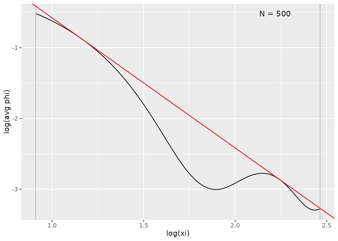

The legend labels each line:

Empirical |phi|: the empirical Fourier transform magnitude
Fitted envelope: the fitted envelope \(A|\xi|^{-r}\), drawn over the selected window
Shaded band: the frequency range used for fitting

Constructing the bias bound

Given the smoothness envelope, the largest possible bias at \(x\) is

\[\bar{b}(x) = \int_{-\infty}^{\infty} |K^{FT}(h\xi) - 1| \cdot A |\xi|^{-r} d\xi,\]

which can be computed analytically for many kernels. This \(\bar{b}\) is the worst-case bias consistent with the detected smoothness, and the true bias satisfies

\[|E[\hat{f}_h(x)] - f(x)| \leq \bar{b}(x).\]

A textbook confidence interval ignores the bias,

\[CI_{\text{naive}} = \hat{f}(x) \pm z_{\alpha/2} \hat{\sigma}(x),\]

so its coverage is wrong when the bias is non-negligible. The bias-bound interval adds the bound on both sides,

\[CI_{\text{bias-bound}} = [\hat{f}(x) - \bar{b}(x) - z_{\alpha/2}\hat{\sigma}(x), \quad \hat{f}(x) + \bar{b}(x) + z_{\alpha/2}\hat{\sigma}(x)],\]

accounting for the worst-case bias in both directions:

# The plot shows both bands
plot(fit)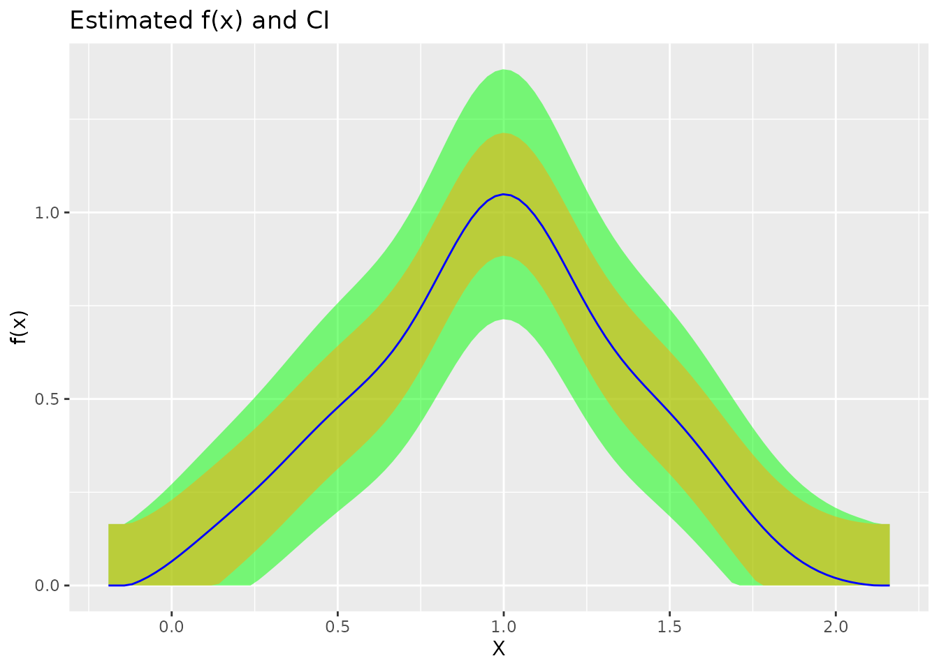

The legend labels the two bands:

Bias bound: the bias range \([\hat{f} - \bar{b}, \hat{f} + \bar{b}]\)
95% CI: the full confidence interval including sampling uncertainty

Kernels

For the bias-bound approach, infinite-order kernels are recommended because they satisfy

\[K^{FT}(\xi) = 1 \text{ for } |\xi| \leq 1,\]

which means no bias from frequencies below \(1/h\) and a simpler bias-bound calculation. Four kernels are available:

Kernel	Order	Fourier Transform
Schennach2004	\(\infty\)	Smooth transition at \(\|\xi\|=1\)
sinc	\(\infty\)	Sharp cutoff at \(\|\xi\|=1\)
normal	2	Gaussian decay
epanechnikov	2	Finite support

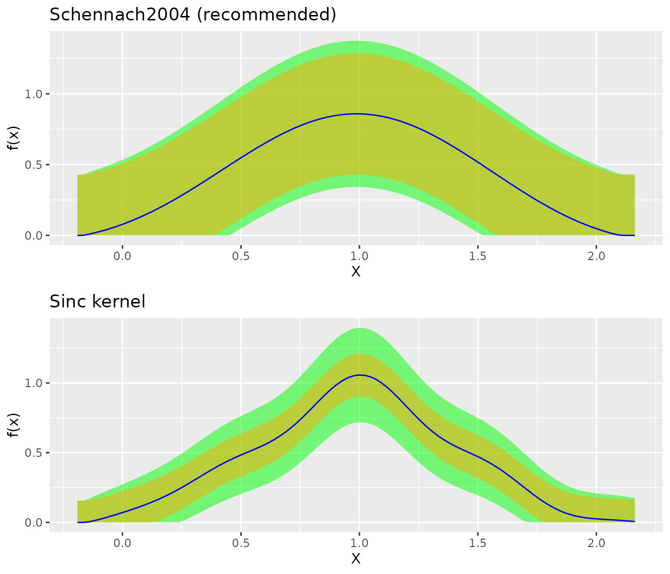
library(gridExtra)

fit_sch <- biasBound_density(X, kernel.fun = "Schennach2004")
fit_sinc <- biasBound_density(X, kernel.fun = "sinc")

grid.arrange(
  plot(fit_sch) + ggtitle("Schennach2004 (recommended)"),
  plot(fit_sinc) + ggtitle("Sinc kernel"),
  ncol = 1
)

Extension to regression

The same principles apply to regression. For \(E[Y \mid X = x]\) the Nadaraya-Watson estimator is

\[\hat{m}(x) = \frac{\sum_{i=1}^{n} K_h(x - X_i) Y_i}{\sum_{i=1}^{n} K_h(x - X_i)},\]

and its bias can be bounded using the Fourier representation of the conditional expectation function:

# Generate regression data
Y <- sin(2 * pi * X) + rnorm(500, sd = 0.3)

# Estimate with bias bounds
fit_reg <- biasBound_condExpectation(Y, X, h = 0.1)

# View smoothness parameters
coef(fit_reg)
#>          A          r          B          h 
#> 22.9169202  2.0000000  0.6374611  0.1000000

Bandwidth selection

The bandwidth is chosen by ordinary least-squares (leave-one-out) cross-validation, the same MSE-minimizing criterion used in standard kernel density estimation. This step is entirely separate from the Fourier analysis above: cross-validation selects the bandwidth, and the Fourier envelope is used only afterwards to bound the bias at that bandwidth.

\[h_{CV} = \arg\min_h \left[ \int \hat{f}_h(x)^2 \, dx \;-\; \frac{2}{n} \sum_{i=1}^{n} \hat{f}_{-i,h}(X_i) \right]\]

where \(\hat{f}_{-i,h}\) is the estimate computed without observation \(i\).

h_cv <- select_bandwidth(X, method = "cv", kernel.fun = "Schennach2004")
h_silv <- select_bandwidth(X, method = "silverman", kernel.fun = "normal")

cat("CV bandwidth:", round(h_cv, 4), "\n")
#> CV bandwidth: 0.2508
cat("Silverman bandwidth:", round(h_silv, 4))
#> Silverman bandwidth: 0.1045

At the MSE-optimal (cross-validation) bandwidth the bias is large enough to matter. The kernel rounds off peaks and other curvature, so the estimate is systematically off there. A textbook confidence interval, the estimate plus or minus a multiple of its standard deviation, ignores this bias and is therefore invalid at the optimal bandwidth. The bias bound addresses this directly: it widens the interval by the worst-case bias and restores valid coverage without changing the bandwidth.

The figure below makes this concrete at the optimal bandwidth. The narrow band is the naive interval (standard deviation only); the wider band is the bias-bound interval. Near the peak the true density (dashed line) leaves the naive band but stays inside the bias-bound band:

fit_opt <- biasBound_density(X, h = h_cv, kernel.fun = "Schennach2004")

# True density: the convolution of two U[0,1] is the triangular density on [0, 2]
tri_density <- function(x) ifelse(x >= 0 & x <= 2, 1 - abs(x - 1), 0)

z <- qnorm(0.975)
band_df <- data.frame(
  x        = fit_opt$x,
  estimate = fit_opt$density,
  truth    = tri_density(fit_opt$x),
  naive_lo = pmax(fit_opt$density - z * fit_opt$std_error, 0),
  naive_hi = fit_opt$density + z * fit_opt$std_error,
  bb_lo    = fit_opt$conf_int$lower,
  bb_hi    = fit_opt$conf_int$upper
)

ggplot(band_df, aes(x)) +
  geom_ribbon(aes(ymin = bb_lo, ymax = bb_hi, fill = "Bias-bound 95% CI")) +
  geom_ribbon(aes(ymin = naive_lo, ymax = naive_hi, fill = "Naive 95% CI (ignores bias)")) +
  geom_line(aes(y = estimate, color = "Estimate"), linewidth = 0.7) +
  geom_line(aes(y = truth, color = "True density"), linetype = "dashed", linewidth = 0.7) +
  scale_fill_manual(values = c("Bias-bound 95% CI" = "#9ECAE1",
                               "Naive 95% CI (ignores bias)" = "#FCAE91")) +
  scale_color_manual(values = c("Estimate" = "#08306B", "True density" = "black")) +
  labs(x = "x", y = "density", fill = NULL, color = NULL) +
  theme(legend.position = "top")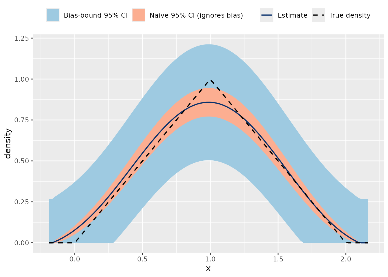

So why prefer the optimal bandwidth at all, given that the bias bound makes its band wider? The classical route to valid inference is undersmoothing: shrink the bandwidth until the bias is small enough to ignore. That restores validity too, but it inflates the variance, and the inflation grows without bound as the sample size increases (the mean squared error of an undersmoothed estimator is asymptotically infinitely larger than at the optimal bandwidth). The bias-bound interval keeps the optimal variance rate and pays a one-time, explicitly bounded price for the bias. Schennach (2020) shows the bias-bound bands are therefore asymptotically shorter than the undersmoothed bands needed for valid classical inference. Their coverage is deliberately conservative, so in a finite sample the band can be wider than the bias actually warrants, and here it is wider than a moderately undersmoothed band.

Summary

The bias-bound approach provides:

Valid inference with optimal bandwidths
Automatic smoothness detection via Fourier analysis
Explicit bias accounting in confidence intervals
Efficiency gains over undersmoothing

References

Schennach, S. M. (2020). A Bias Bound Approach to Non-parametric Inference. The Review of Economic Studies, 87(5), 2439-2472. doi:10.1093/restud/rdz065