Bias bound approach for conditional expectation estimation
biasBound_condExpectation.RdEstimates the density at a given point or across a range, and provides visualization options for density, bias, and confidence intervals.
Usage
biasBound_condExpectation(
  Y,
  X,
  x = NULL,
  h = NULL,
  h_method = "cv",
  alpha = 0.05,
  est_Ar = NULL,
  resol = 100,
  xi_lb = NULL,
  xi_ub = NULL,
  methods_get_xi = "snr",
  noise_floor = "auto",
  envelope_use_Y = TRUE,
  integer_r = TRUE,
  ora_Ar = NULL,
  kernel.fun = "Schennach2004",
  if_approx_kernel = TRUE,
  kernel.resol = 1000
)
Arguments
- Y
A numerical vector of sample data.
- X
A numerical vector of sample data.
- x
Optional. A scalar or range of points where the density is estimated. If NULL, a range is automatically generated.
- h
A scalar bandwidth parameter. If NULL, the bandwidth is automatically selected using the method specified in 'h_method'.
- h_method
Method for automatic bandwidth selection when h is NULL. Options are "cv" (cross-validation) and "silverman" (Silverman's rule of thumb). Default is "cv".
- alpha
Confidence level for intervals. Default is 0.05.
- est_Ar
Optional list of estimates for A and r. If NULL, they are computed using
get_est_Ar().- resol
Resolution for the estimation range. Default is 100.
- xi_lb
Optional. Lower bound for the interval of Fourier Transform frequency xi. Used for determining the range over which A and r is estimated. If NULL, it is automatically determined based on the methods_get_xi.
- xi_ub
Optional. Upper bound for the interval of Fourier Transform frequency xi. Similar to xi_lb, it defines the upper range for A and r estimation. If NULL, the upper bound is determined based on the methods_get_xi.
- methods_get_xi
A string selecting the frequency-window rule used when xi_lb/xi_ub are NULL: "snr" (default; a signal-to-noise cutoff that selects a valid window at realistic sample sizes), "Schennach" (the data-driven rule of Schennach 2020, Theorem 2), or "Schennach_loose" (the initial, un-refined interval).
- noise_floor
Noise-floor form for the Schennach test: "auto" (default), "compact", or "general".
- envelope_use_Y
If TRUE (default), fit the regression envelope to the cross-spectrum
|phi_YX|; if FALSE, fit it to the marginal spectrum|phi_X|.- integer_r
If TRUE (default), clamp the fitted envelope slope up to r = 2 when it falls below the minimum smoothness assumed by Schennach (2020, Definition 2), i.e. r < 2, and refit A; this keeps the bias-bound integral finite. Slopes >= 2 are left unchanged.
- ora_Ar
Optional list of oracle values for A and r (for research/comparison purposes).
- kernel.fun
A string specifying the kernel function to be used. Options are "Schennach2004", "sinc", "normal", "epanechnikov".
- if_approx_kernel
Logical. If TRUE, uses approximations for the kernel function.
- kernel.resol
The resolution for kernel function approximation. See
fun_approx.
Value
An object of class bbnp_regression with components:
- fitted_values
\(E[Y|X=x]\) estimates (for range estimation)
- x
Evaluation points
- estimate
Point estimate (for single x)
- conf_int
List containing lower, upper bounds and conf_level. Note that the confidence interval can be unbounded (i.e., contain
-InforInf) in regions where the estimated marginal density \(\hat f(x)\) is very close to zero, because the estimator is formed as a ratio involving \(1/\hat f(x)\).- bias_bound
List containing b1x, byx, est_A, est_r, est_B, xi_interval
- std_error
Standard errors
- marginal_density
f(x) estimates
- joint_density
f_YX estimates
- call
The function call
- bandwidth
Bandwidth used
- n
Sample size
- kernel
Kernel type
- data
Original data (X, Y)
Use plot(), summary(), coef(), fitted(), and confint() methods to work with the result.
Examples
# \donttest{
# Example 1: Point estimation at x = 1
X <- gen_sample_data(size = 500, dgp = "2_fold_uniform", seed = 1)
Y <- 2 * X - X^2 + rnorm(length(X), sd = 0.3)
fit <- biasBound_condExpectation(Y = Y, X = X, x = 1, h = 0.09)
print(fit)
#> Bias-Bounded Conditional Expectation Estimation
#>
#> Call:
#> biasBound_condExpectation(Y = Y, X = X, x = 1, h = 0.09)
#>
#> Sample size: n = 500
#> Bandwidth: h = 0.0900 (user-specified)
#> Kernel: Schennach2004
#>
#> Bias bound parameters:
#> A = 4.4348, r = 2.0000, B = 0.8231
#> bias bounds: b1x = 0.0000, byx = 0.1307
#>
#> Point estimate at x = 1.0000: E[Y|X=x] = 0.9987
#> Confidence level: 95%
#>
#> Use summary() for detailed statistics
#> Use plot() to visualize results
#> Use fitted() to extract fitted values
fitted(fit)
#> [1] 0.998705
# Example 2: Range estimation with plots
fit2 <- biasBound_condExpectation(Y = Y, X = X, h = NULL, h_method = "cv")
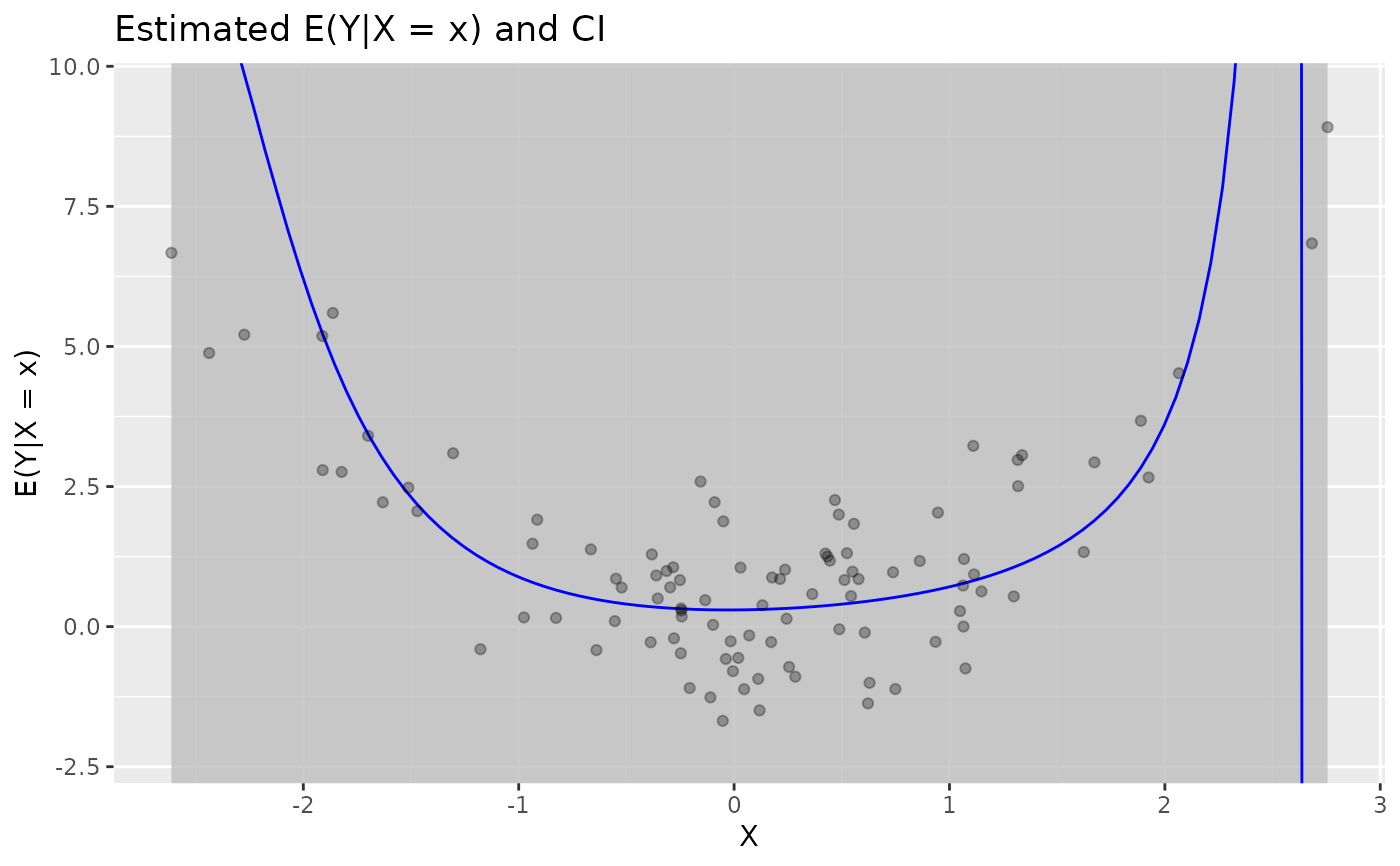
plot(fit2) # Regression plot
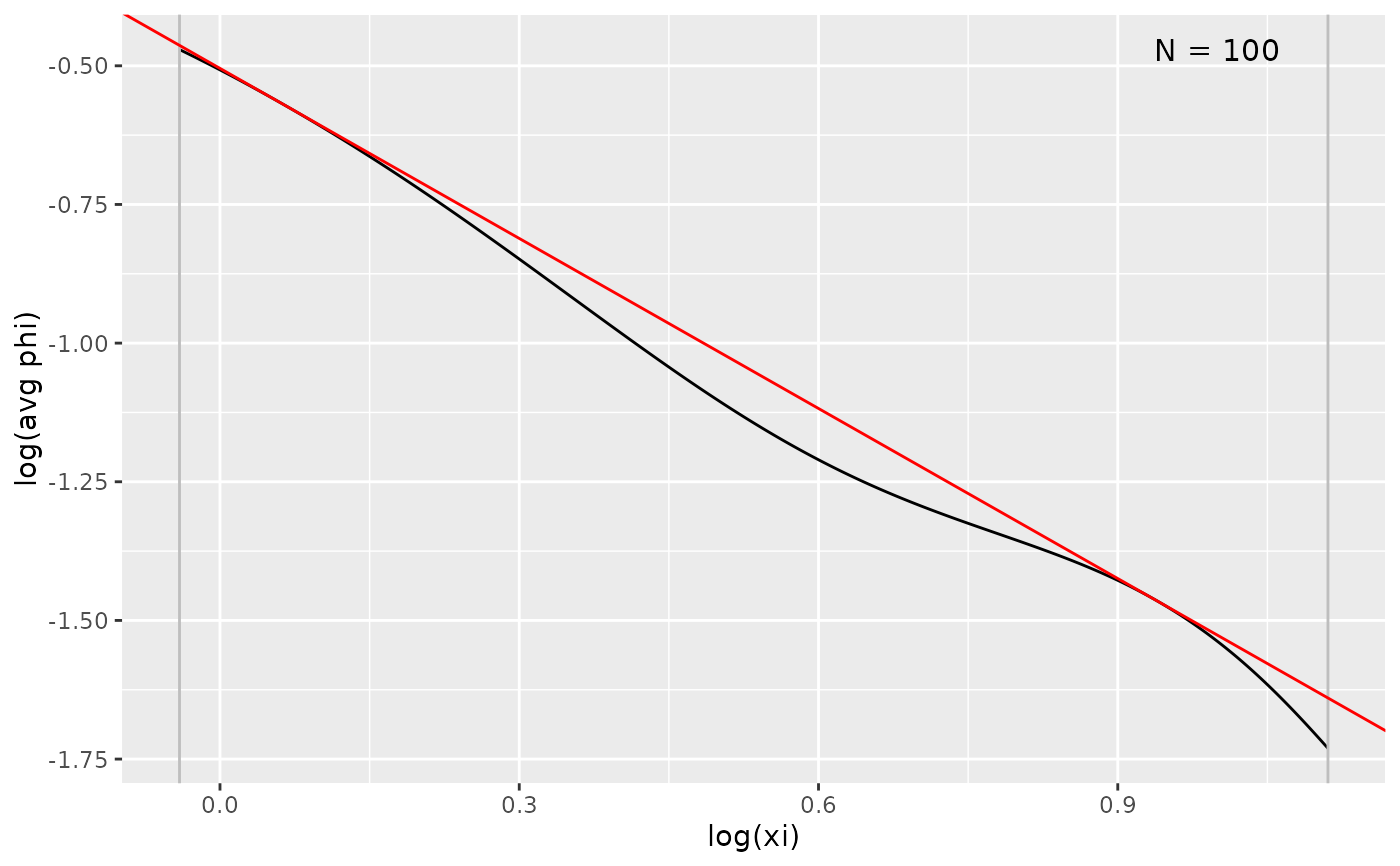
 plot(fit2, type = "ft") # Fourier transform plot
 summary(fit2)
#> Summary: Bias-Bounded Conditional Expectation Estimation
#> ============================================================
#>
#> Call:
#> biasBound_condExpectation(Y = Y, X = X, h = NULL, h_method = "cv")
#>
#> Sample Information:
#> Sample size (n): 500
#> Bandwidth (h): 0.2603
#> Kernel function: Schennach2004
#>
#> Bias Bound Parameters:
#> A (amplitude): 4.4348
#> r (decay rate): 2.0000
#> B (Y bound): 0.8231
#> b1x (bias f(x)): 0.0000
#> byx (bias f_YX): 0.3780
#> Xi interval: [2.3941, 5.3114]
#>
#> Range Estimation:
#> Fitted values (E[Y|X]):
#> min Q1.25% median mean Q3.75% max
#> 0.4481 0.7389 0.8435 0.7993 0.8935 0.9087
#>
#> Marginal density f(x):
#> min mean max
#> 0.1418 0.5338 0.8132
#>
#> Standard errors:
#> min mean max
#> 0.0067 0.0114 0.0136
#>
# }
summary(fit2)
#> Summary: Bias-Bounded Conditional Expectation Estimation
#> ============================================================
#>
#> Call:
#> biasBound_condExpectation(Y = Y, X = X, h = NULL, h_method = "cv")
#>
#> Sample Information:
#> Sample size (n): 500
#> Bandwidth (h): 0.2603
#> Kernel function: Schennach2004
#>
#> Bias Bound Parameters:
#> A (amplitude): 4.4348
#> r (decay rate): 2.0000
#> B (Y bound): 0.8231
#> b1x (bias f(x)): 0.0000
#> byx (bias f_YX): 0.3780
#> Xi interval: [2.3941, 5.3114]
#>
#> Range Estimation:
#> Fitted values (E[Y|X]):
#> min Q1.25% median mean Q3.75% max
#> 0.4481 0.7389 0.8435 0.7993 0.8935 0.9087
#>
#> Marginal density f(x):
#> min mean max
#> 0.1418 0.5338 0.8132
#>
#> Standard errors:
#> min mean max
#> 0.0067 0.0114 0.0136
#>
# }