Get Started with rbbnp
rbbnp.RmdOverview
The rbbnp package implements the bias-bound approach to nonparametric inference of Schennach (2020). Nonparametric inference faces a long-standing dilemma. At the bandwidth that minimizes mean squared error the estimator carries a non-negligible bias, which invalidates the usual confidence intervals. Undersmoothing removes that bias but widens the intervals and sacrifices efficiency. The bias-bound approach keeps the optimal bandwidth and estimates an upper bound on the magnitude of the bias, then builds that bound into the interval:
\[CI = [\hat{f} - \bar{b} - z_{\alpha/2}\hat{\sigma}, \quad \hat{f} + \bar{b} + z_{\alpha/2}\hat{\sigma}]\]
where \(\bar{b}\) is the estimated bias bound. The result is a valid confidence interval at the MSE-optimal bandwidth.
Installation
# Install from CRAN
install.packages("rbbnp")

# Or install development version from GitHub
# install.packages("devtools")
devtools::install_github("xinyu-daidai/rbbnp-dev")
Quick Start
Density Estimation
# Generate sample data
X <- gen_sample_data(size = 500, dgp = "2_fold_uniform", seed = 123456)

# Estimate density with bias-aware confidence intervals
fit <- biasBound_density(X, h = 0.1, kernel.fun = "Schennach2004")

# View summary
fit
#> Bias-Bounded Density Estimation
#>
#> Call:
#> biasBound_density(X = X, h = 0.1, kernel.fun = "Schennach2004")
#>
#> Sample size: n = 500
#> Bandwidth:   h = 0.1000 (user-specified)
#> Kernel:      Schennach2004
#>
#> Bias bound parameters:
#>   A = 6.3312, r = 2.3422
#>   bias bound b1x = 0.0714
#>
#> Evaluation points: 100 (range: [-0.1639, 2.0517])
#> Confidence level: 95%
#>
#> Use summary() for detailed statistics
#> Use plot() to visualize results
# Visualize results
plot(fit)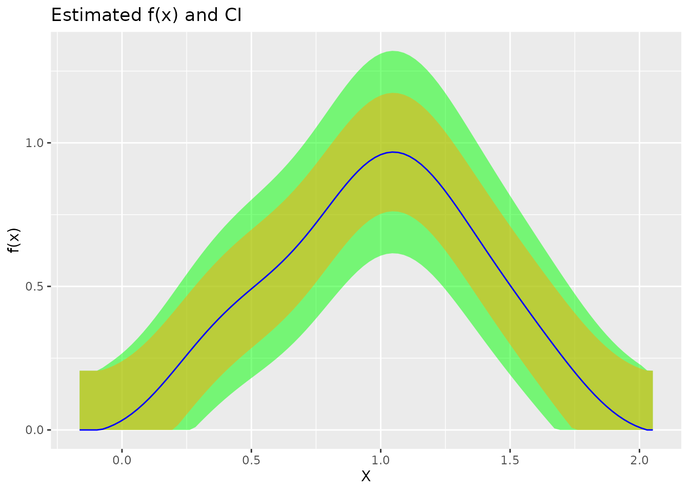
The plot shows (the legend labels each element):
- Estimate: the estimated density \(\hat{f}(x)\)
- Bias bound: the range where \(E[\hat{f}]\) may lie
- 95% CI: the confidence interval
Conditional Expectation (Regression)
# Generate regression data: Y = -X^2 + 3X + noise
Y <- -X^2 + 3*X + rnorm(500) * X

# Estimate conditional expectation
fit_reg <- biasBound_condExpectation(Y, X, h = 0.1, kernel.fun = "Schennach2004")

# Visualize
plot(fit_reg)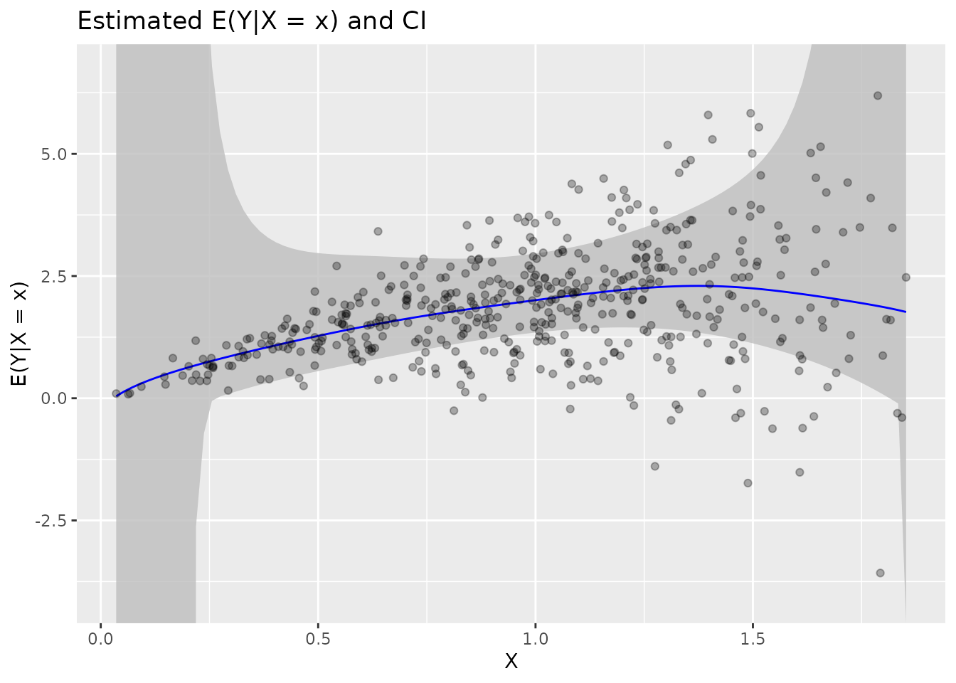
Working with Results
Both functions return S3 objects with standard methods:
# Extract parameters
coef(fit)
#>      A      r      h
#> 6.3312 2.3422 0.1000

# Get confidence intervals
head(confint(fit))
#>      lower      upper
#> [1,]     0 0.07139636
#> [2,]     0 0.07139636
#> [3,]     0 0.07139636
#> [4,]     0 0.07139636
#> [5,]     0 0.08205420
#> [6,]     0 0.09605150

# For regression: get fitted values
head(fitted(fit_reg))
#> [1] 0.0420927 0.1386661 0.2211023 0.2938845 0.3597238 0.4202832
Next Steps
- Density Estimation: Detailed guide to density estimation
- Regression: Conditional expectation estimation
- Theory: Mathematical background
References
Schennach, S. M. (2020). A Bias Bound Approach to Non-parametric Inference. The Review of Economic Studies, 87(5), 2439-2472. doi:10.1093/restud/rdz065