Regression with rbbnp
regression.RmdThis article is a guide to conditional expectation (regression)
estimation with biasBound_condExpectation().
Estimating a conditional expectation
biasBound_condExpectation() estimates \(E[Y \mid X = x]\) with bias-aware
confidence intervals. Its main arguments are:
biasBound_condExpectation(
  Y,                    # Response variable
  X,                    # Predictor variable
  x = NULL,             # Evaluation points
  h = NULL,             # Bandwidth
  h_method = "cv",      # "cv" or "silverman"
  alpha = 0.05,         # Confidence level
  kernel.fun = "Schennach2004"
)
A basic fit, on data with a quadratic mean and Gaussian noise:
# Generate data: Y = f(X) + noise
set.seed(42)
X <- gen_sample_data(size = 800, dgp = "2_fold_uniform")
Y <- 2 * X - X^2 + rnorm(800, sd = 0.3)

# Estimate conditional expectation E[Y|X]
fit <- biasBound_condExpectation(Y, X, h = 0.1, kernel.fun = "Schennach2004")

# View results
fit
#> Bias-Bounded Conditional Expectation Estimation
#>
#> Call:
#> biasBound_condExpectation(Y = Y, X = X, h = 0.1, kernel.fun = "Schennach2004")
#>
#> Sample size: n = 800
#> Bandwidth:   h = 0.1000 (user-specified)
#> Kernel:      Schennach2004
#>
#> Bias bound parameters:
#>   A = 4.9135, r = 2.0000, B = 0.8374
#>   bias bounds: b1x = 0.0000, byx = 0.1609
#>
#> Evaluation points: 100 (range: [0.0688, 1.9084])
#> Fitted values: E[Y|X] range [0.2421, 1.0004]
#> Confidence level: 95%
#>
#> Use summary() for detailed statistics
#> Use plot() to visualize results
#> Use fitted() to extract fitted values
The fit is an S3 object of class bbnp_regression. Use
coef() for the key parameters and summary()
for a fuller report:
# Key parameters
coef(fit)
#>         A         r         B         h
#> 4.9135200 2.0000000 0.8374278 0.1000000

# Detailed summary
summary(fit)
#> Summary: Bias-Bounded Conditional Expectation Estimation
#> ============================================================
#>
#> Call:
#> biasBound_condExpectation(Y = Y, X = X, h = 0.1, kernel.fun = "Schennach2004")
#>
#> Sample Information:
#>   Sample size (n):  800
#>   Bandwidth (h):    0.1000
#>   Kernel function:  Schennach2004
#>
#> Bias Bound Parameters:
#>   A (amplitude):    4.9135
#>   r (decay rate):   2.0000
#>   B (Y bound):      0.8374
#>   b1x (bias f(x)):  0.0000
#>   byx (bias f_YX):  0.1609
#>   Xi interval:      [2.4522, 6.0820]
#>
#> Range Estimation:
#>   Fitted values (E[Y|X]):
#>    min Q1.25% median   mean Q3.75%    max
#> 0.2421 0.5279 0.7689 0.7219 0.9413 1.0004
#>
#>   Marginal density f(x):
#>    min   mean    max
#> 0.0911 0.5333 0.9695
#>
#>   Standard errors:
#>    min   mean    max
#> 0.0057 0.0127 0.0183
Visualizing the fit
The default plot shows the estimated mean, its confidence band, and the original data:
plot(fit)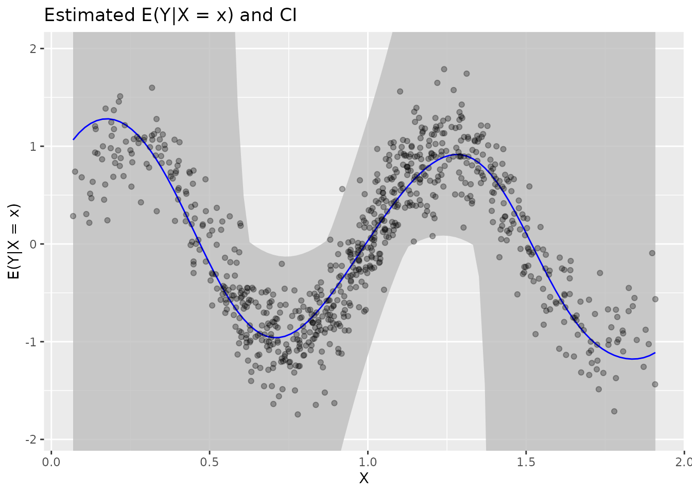
| Element | Description |
|---|---|
| Estimate (line) | Estimated \(\hat{E}[Y \mid X=x]\) |
| 95% CI (band) | Confidence interval |
| Points | Original data \((X_i, Y_i)\) |
Because the plot returns a ggplot object, you can overlay the true mean for comparison:
# True function for comparison
true_fn <- function(x) 2 * x - x^2

plot(fit) +
  stat_function(fun = true_fn, aes(color = "True E[Y|X]"),
                linetype = "dashed", linewidth = 1) +
  scale_color_manual(values = c("Estimate" = "#08306B", "True E[Y|X]" = "red")) +
  labs(color = NULL) +
  theme(legend.position = "top")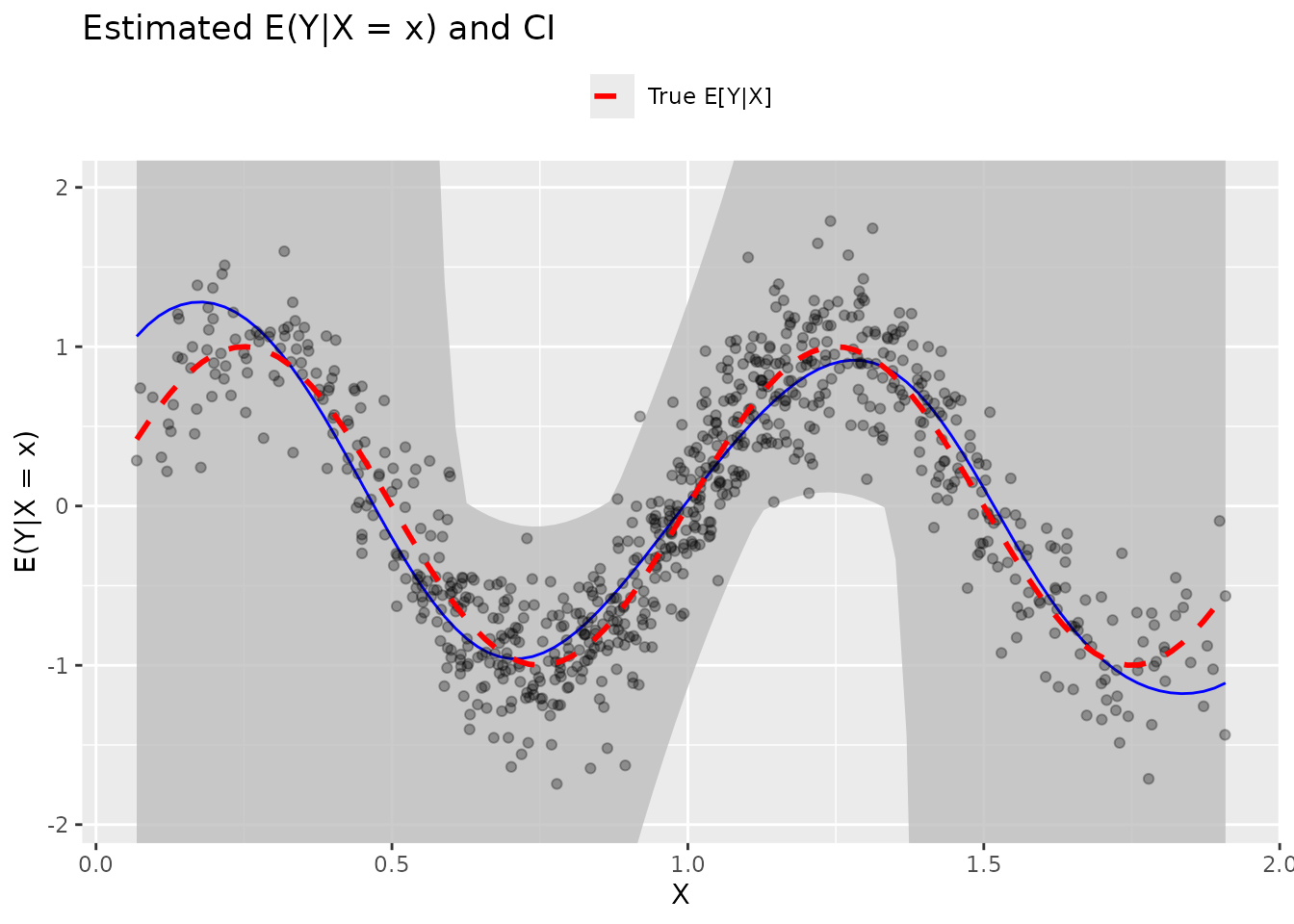
Fitted values and confidence intervals
fitted() returns the estimated mean at the evaluation
points:
# Get fitted values at evaluation points
predictions <- fitted(fit)
head(predictions, 10)
#>  [1] 0.2754944 0.2951673 0.3146228 0.3340021 0.3534049 0.3729038 0.3924839
#>  [8] 0.4121796 0.4319836 0.4519014

# Evaluation points
x_points <- fit$x
head(x_points)
#> [1] 0.06877618 0.08735791 0.10593964 0.12452137 0.14310310 0.16168483
In regions where the estimated marginal density \(\hat f(x)\) is very close to zero, the
confidence interval may become unbounded (it can contain
-Inf or Inf). This happens because the
conditional mean estimator is a ratio involving \(1/\hat f(x)\). The interval is finite at
interior points, where the density is well away from zero:
# Extract confidence intervals
ci <- confint(fit)

# Show the interval at interior points, where the marginal density is well away
# from zero so the ratio-based interval is finite
ok <- which(is.finite(ci[, "lower"]) & is.finite(ci[, "upper"]))
data.frame(
  x = fit$x[ok],
  estimate = fitted(fit)[ok],
  lower = ci[ok, "lower"],
  upper = ci[ok, "upper"]
)[1:6, ]
#>            x  estimate      lower    upper
#> 1 0.06877618 0.2754944 -1.2548307 1.805820
#> 2 0.08735791 0.2951673 -1.0500228 1.640357
#> 3 0.10593964 0.3146228 -0.8814441 1.510690
#> 4 0.12452137 0.3340021 -0.7401813 1.408186
#> 5 0.14310310 0.3534049 -0.6197525 1.326562
#> 6 0.16168483 0.3729038 -0.5155217 1.261329
Choosing the bandwidth
When h is NULL, the bandwidth is selected
automatically. Cross-validation is the default:
fit_cv <- biasBound_condExpectation(Y, X, h = NULL, h_method = "cv")
cat("CV bandwidth:", coef(fit_cv)["h"])
#> CV bandwidth: 0.2313533
Silverman’s rule is a faster alternative:
fit_silv <- biasBound_condExpectation(Y, X, h = NULL, h_method = "silverman")
cat("Silverman bandwidth:", coef(fit_silv)["h"])
#> Silverman bandwidth: 0.1156766
Worked examples
Built-in sample data
# Load sample data
data(sample_data)
head(sample_data)
#>           X        Y
#> 1 1.0859914 2.828175
#> 2 1.6292714 2.014698
#> 3 1.2303920 3.350186
#> 4 1.0686912 1.953532
#> 5 0.8441481 1.391845
#> 6 0.8789330 1.954778

# Estimate regression
fit_real <- biasBound_condExpectation(
  Y = sample_data$Y,
  X = sample_data$X,
  h = 0.1,
  kernel.fun = "Schennach2004"
)

# Visualize
plot(fit_real) + ggtitle("Regression on Sample Data")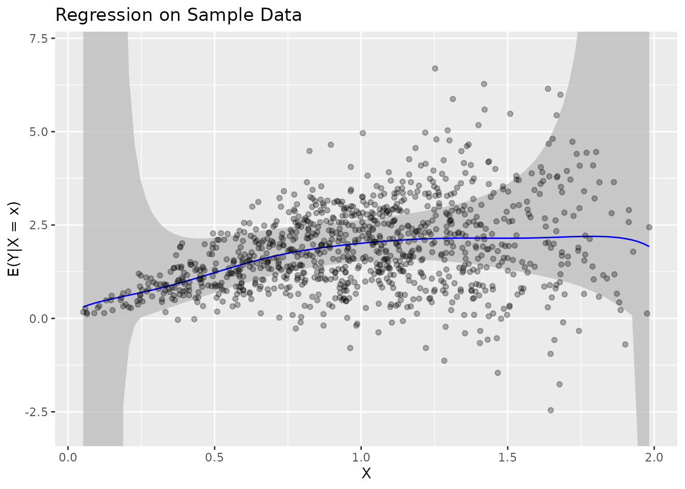
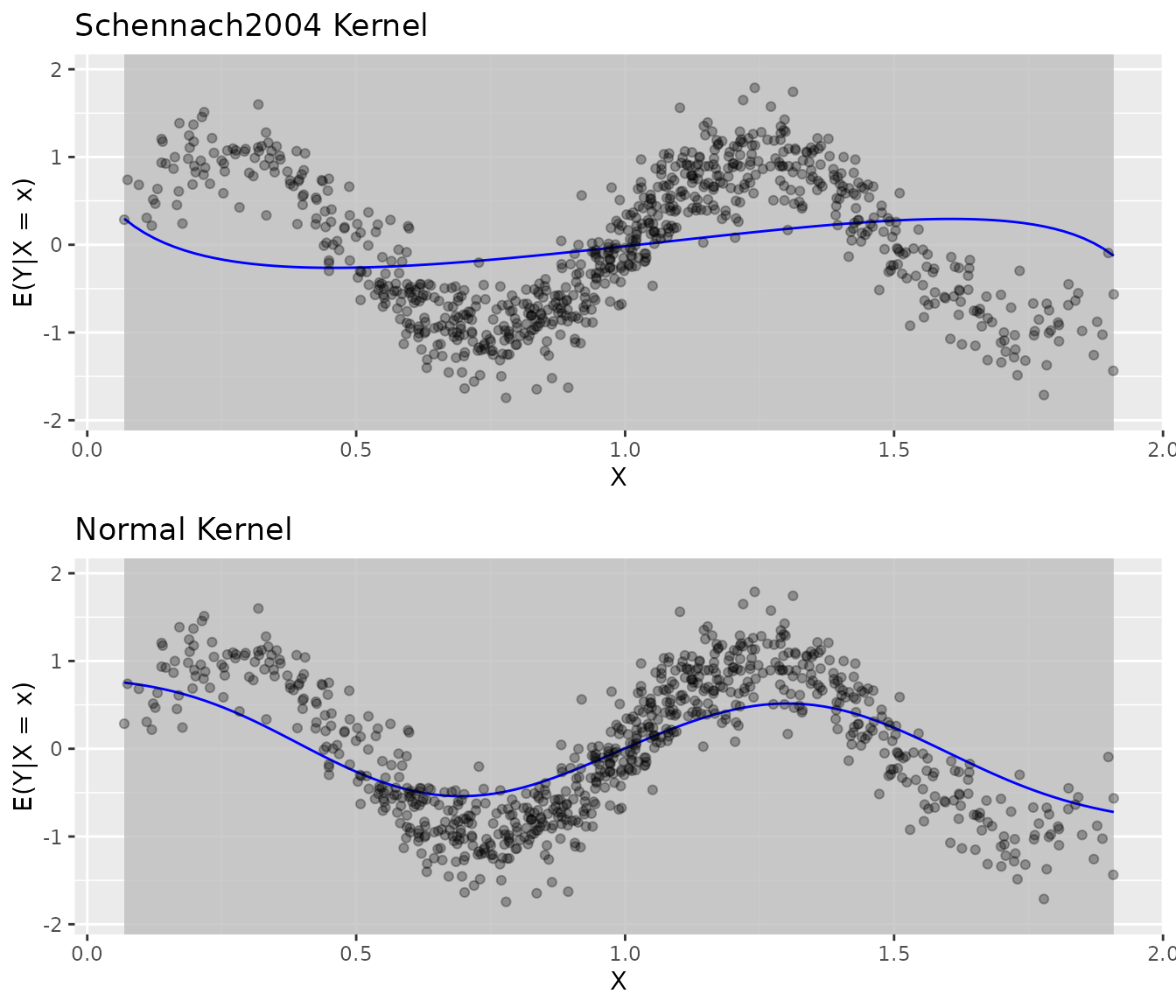
Comparing kernels
fit_sch <- biasBound_condExpectation(Y, X, h = 0.1, kernel.fun = "Schennach2004")
fit_norm <- biasBound_condExpectation(Y, X, h = 0.1, kernel.fun = "normal")

grid.arrange(
  plot(fit_sch) + ggtitle("Schennach2004 Kernel"),
  plot(fit_norm) + ggtitle("Normal Kernel"),
  ncol = 1
)
Heteroscedastic errors
The method handles errors whose variance changes with
X:
# Generate heteroscedastic data
set.seed(123)
X_het <- gen_sample_data(size = 600, dgp = "2_fold_uniform")
Y_het <- X_het^2 + rnorm(600) * X_het  # Variance increases with X

fit_het <- biasBound_condExpectation(Y_het, X_het, h = 0.1)
plot(fit_het) + ggtitle("Heteroscedastic Data")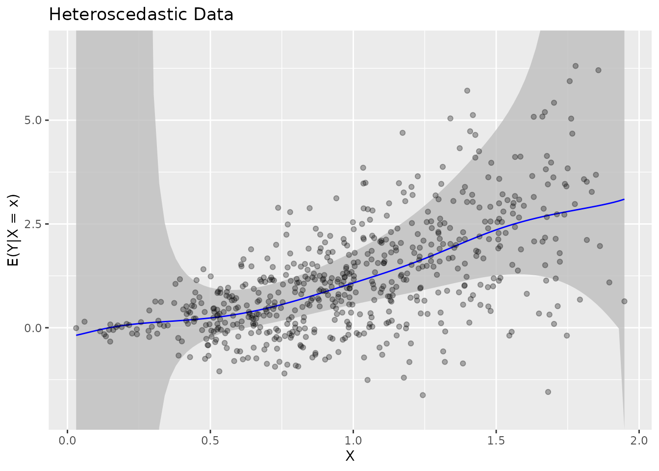
A polynomial mean
# Quadratic relationship
set.seed(456)
X_poly <- gen_sample_data(size = 500, dgp = "2_fold_uniform")
Y_poly <- -X_poly^2 + 3*X_poly + rnorm(500, sd = 0.5)

fit_poly <- biasBound_condExpectation(Y_poly, X_poly, h = 0.1)

# Compare with true function
true_poly <- function(x) -x^2 + 3*x

plot(fit_poly) +
  stat_function(fun = true_poly, aes(color = "True: -x^2 + 3x"),
                linetype = "dashed", linewidth = 1) +
  scale_color_manual(values = c("Estimate" = "#08306B", "True: -x^2 + 3x" = "red")) +
  labs(color = NULL) +
  theme(legend.position = "top")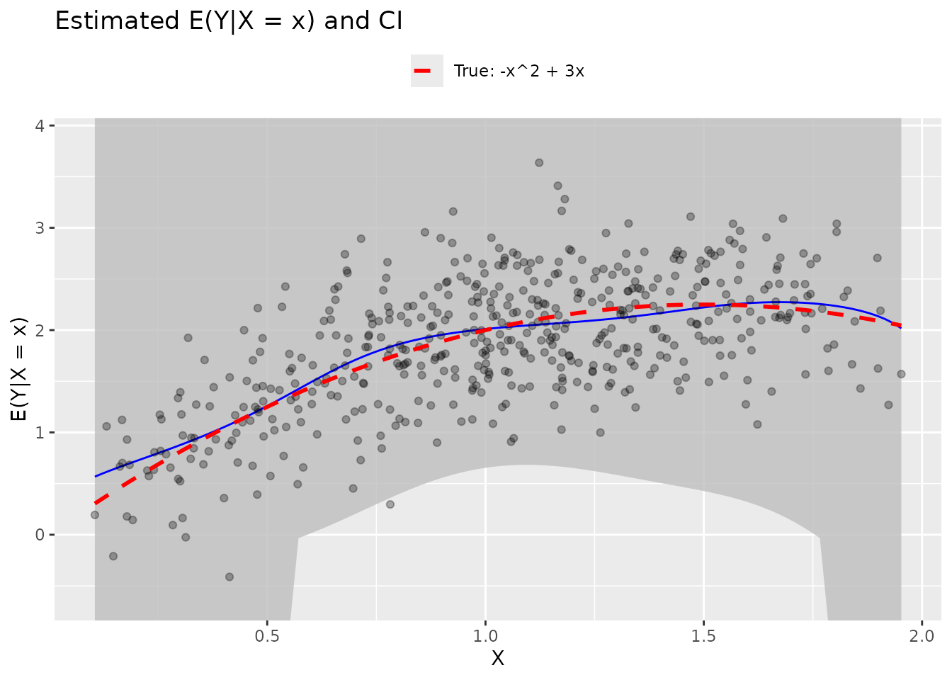
See Also
- Get Started: Quick introduction
- Density Estimation: Density estimation details
- Theory: Mathematical background